
GIMP
News
Docs
Tutorials
More
A very common editing problem is how to lighten the shadows and midtones of an image while retaining highlight details, a task sometimes referred to as “shadow recovery” and more generally speaking as “tone mapping”. This step-by-step tutorial shows you how to use high bit depth GIMP’s floating point “Colors/Exposure” operation to add one or more stops of positive exposure compensation to an image’s shadows and midtones while retaining highlight details.
Page Contents
A very common editing problem is how to lighten the shadows and midtones of an image without blowing out the highlights, which problem is very often encountered when dealing with photographs of scenes lit by direct sunlight. Precanned algorithms for accomplishing this task are often referred to as “shadow recovery” algorithms. But really these algorithms are special-purpose tone-mapping algorithms, which sometimes work pretty well, and sometimes not so well, depending on the algorithm, the image, and your artistic intentions for the image.
This step-by-step tutorial shows you how to use GIMP’s unbounded floating point “Colors/Exposure” operation to recover shadow information—that is, add one or more stops of positive exposure compensation to an image’s shadows and midtones—without blowing out or unduly compressing the image highlights. The procedure is completely “hand-tunable” using masks and layers, and is as close as you can get to non-destructive image editing using high bit depth GIMP 2.9/2.10.
Hight bit depth GIMP is my primary image editor, and I’ve used the procedure described below for the last couple of years as my “go to” way to modify image tonality. The same general procedure can be used to darken as well as lighten portions of an image, again controlling the effect using a layer mask. This isn’t exactly nondestructive editing because at some point you need to make a “New from Visible” layer. But unlike using Curves, using high bit depth GIMP’s floating point “Colors/Exposure” doesn’t clip RGB channel values and allows you to fine-tune the results by modifying and re-modifying the layer mask until you are completely happy with the resulting tonality.
This step-by-step example provides a sample image and is broken down into five steps, starting with downloading the image. Steps 3, 4, and 5 describe the actual procedure, so here’s an overview:
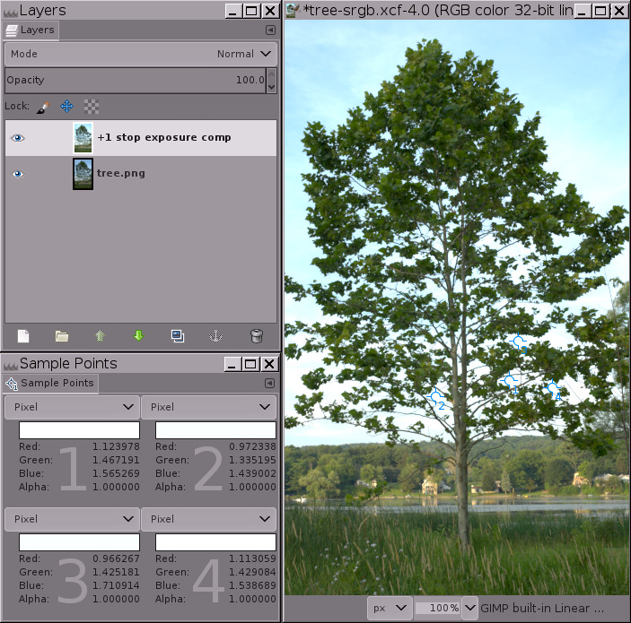
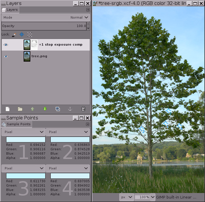
Notice the RGB channel values for the four sample points: the channel information that would have been clipped using integer precision is encoded using channel values that are greater than 1.0 floating point.
The image in Figure 4 clearly has “blown” highlights in the sky. But the highlights aren’t really blown (that is, clipped to 1.0 in one or more channels). Instead the highlight information is still there, but the RGB channel values fall outside the RGB display channel value range of 0.0f to 1.0f. The sample points dialog in Figure 4 above shows four sample points that have RGB channel values that are greater than 1.0. As shown in Figure 5 below, adding a mask allows you to recover these highlights by bringing them back down into the display range.
If you had used integer precision instead of floating point, the highlights really would be blown: The sample points would have a maximum channel values of 255, 65535 or 4294967295, depending on the bit depth. And masking would only “recover” a solid expanse of gray, completely lacking any details (try for yourself and see what happens).
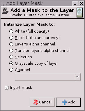 Add an inverse grayscale layer mask: Right-click on the layer and select “Layer/Mask/Add Layer Mask”, and when the “Add a mask to the Layer” dialog pops up, choose “Grayscale copy of layer” and check the “Invert mask” box.
As shown in Figure 5 below, at this point the highlights will be brought back into the display range, meaning all RGB channel values are between 0.0f and 1.0f. But the image will probably look a little odd (sort of cloudy and flat), and depending on the image, the brightest highlights might actually have dark splotches—don’t worry! this is temporary.
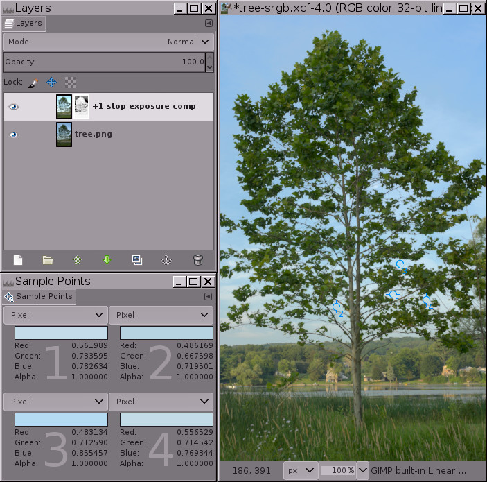
Adding an inverse grayscale layer mask brings the highlights back into the display range, but at this point most images will look flat and cloudy, and some images will have dark splotches in the highlights. The next step—“Auto Stretch Contrast” performed on the mask—will take care of this problem.
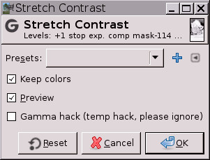 Click on the layer mask to select it for editing, and then select “Colors/Auto/Stretch Contrast”:
“Keep Colors” should be checked (though it doesn’t really matter on grayscale images such as layer masks). Figure 6 below shows the final result:
“Auto/Stretch Contrast” on the mask is necessary because just like the image layer has out of gamut RGB channel values, the inverted grayscale mask contains out of gamut grayscale values. “Auto/Stretch Contrast” brings all the mask grayscale values back into the display range, allowing the mask to proportionately compensate for the layer’s otherwise out-of-gamut RGB channel values, masking more in the layer highlights and less/not at all in the image’s shadows and midtones.
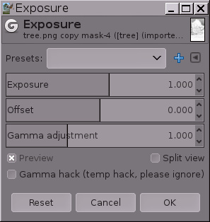
Notice that one of the sample points still has a blue RGB channel value that is slightly out of gamut. The easiest way to deal with this is to “Colors/Exposure” to make a Gamma adjustment of 0.45 on the mask, not on the actual image layer. You can make this Gamma adjustment either on the entire mask (works well, less effort). Or else you can make the adjustment just on the mask shadows (which correspond to the layer highlights), in which case you’d load the mask as a selection, invert the selection, and make the Gamma adjustment. Or if the remaining out of gamut channel values are only very slightly out of gamut, make a “New from Visible” layer and then “Auto/Stretch Contrast” the result to bring the remaining channel values back into gamut.
That’s the whole procedure for using “Colors/Exposure” to add a stop of positive exposure compensation to the shadows without blowing out the highlights. Now you can either fine-tune the mask, or else just make a “New from Visible” layer and continue editing your nicely brightened image. Depending on the image and also on your artistic intentions for the image, the mask might not need fine-tuning. But very often you’ll want to modify the resulting tonal distribution by doing a “Colors/Exposure” gamma correction, or perhaps a Curves operation on the mask, or else by painting directly on the mask. And sometimes you’ll want to blur the mask to restore micro contrast.
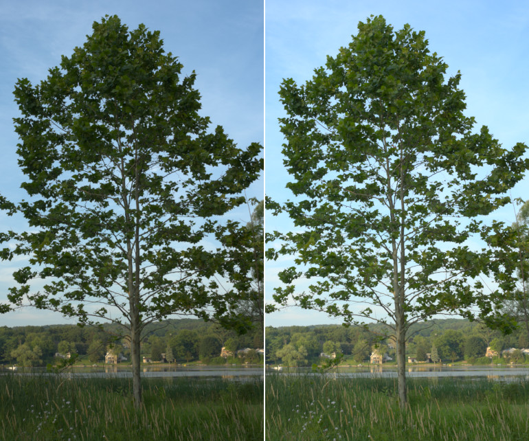
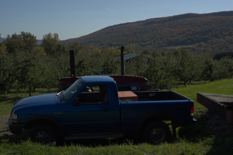 2. After tone mapping/shadow recovery using high bit depth GIMP’s floating point “Colors/Exposure”.
3. For comparison, Mantuik tone-mapping using the GEGL default settings.
2. After tone mapping/shadow recovery using high bit depth GIMP’s floating point “Colors/Exposure”.
3. For comparison, Mantuik tone-mapping using the GEGL default settings.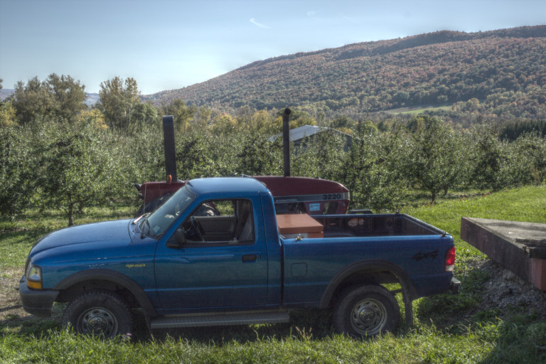
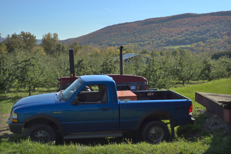
Using GIMP’s floating point “Colors/Exposure” plus layer masks to add two and a half stops of positive exposure compensation to the shadows and midtones of a “bright sun” photograph of an apple orchard truck.
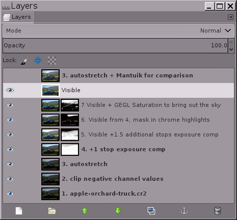 To the right is a screenshot of the layer stack that I used to tone-map the photograph of the apple orchard truck. Tone-mapping by hand gives you complete control over the resulting image. Mantuik and other “automagic” tone-mapping algorithms are CPU-intensive, unpredictable, and often produce unnatural-looking results.
Before using “Colors/Exposure” to add positive exposure compensation, the base layer should already be stretched to its maximum dynamic range. The easiest way to stretch the base layer to its maximum dynamic range is to do “Colors/Auto/Stretch Contrast” and make sure that “Keep colors” is checked.
If you’ve never used an unbounded floating point image editor before, “Colors/Auto/Stretch Contrast” can produce an unexpected result: The image might actually end up with a severely reduced dynamic range, having either lighter shadows or darker highlights or both:
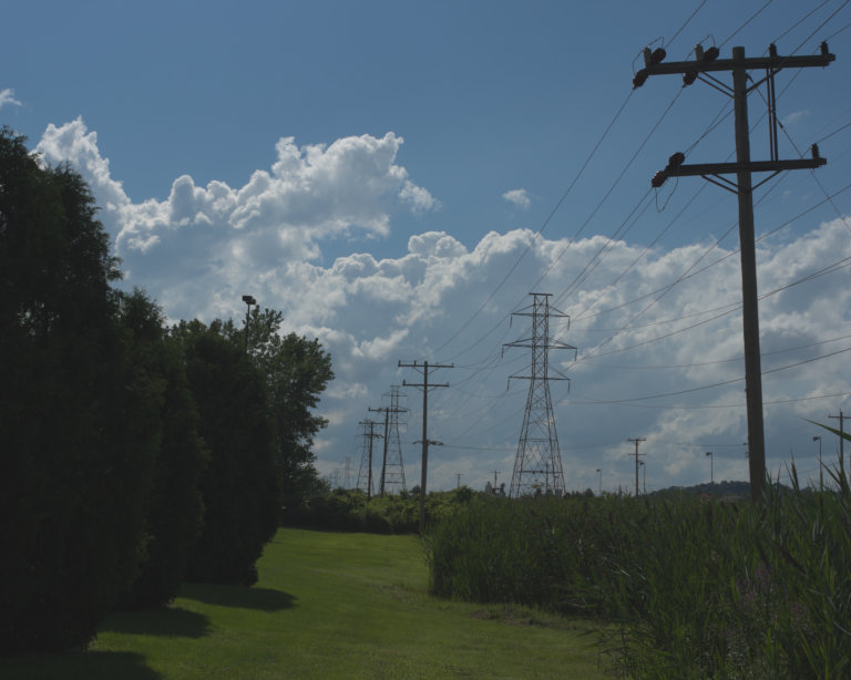
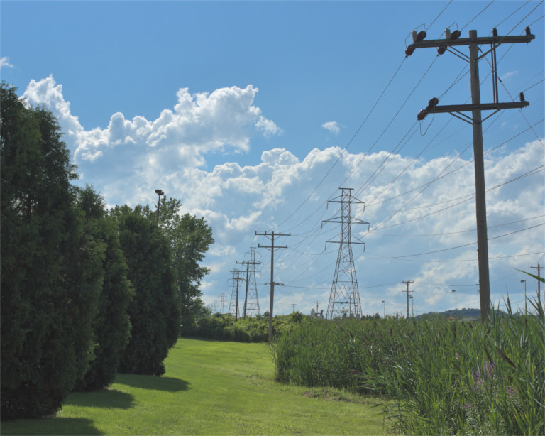
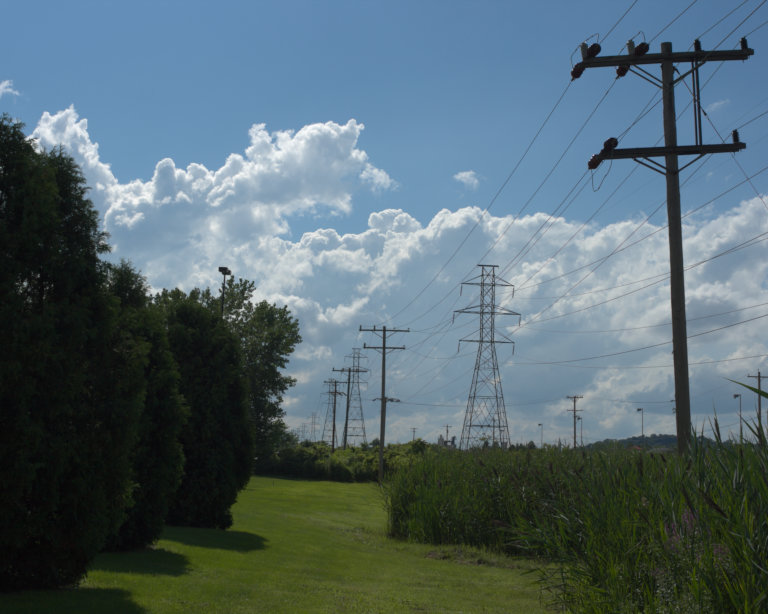
As captured by the raw file, this picture of power lines marching into the distance is a typical result of taking a photograph at noon on a bright sunny day: The sky and clouds looked pretty good right out of the camera, but the ground was far too dark. So the image could benefit from some tone mapping to raise the shadows and midtones. The first step is to do “Colors/Auto/Stretch Contrast” to bring any channel values that are less than 0.0f or greater than 1.0f back within the display range of 0.0 to 1.0 floating point.
Performing “Auto/Stretch Contrast” to bring the channel values back inside the display range doesn’t exactly look like an editing step in the right direction for tone-mapping this particular image! but really it is. Using “Colors/Exposure” to add positive exposure compensation to the shadows and midtones won’t work if the image has channel values that fall outside the display range.
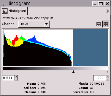 For the “Power lines” picture shown in Figure 8 above, after doing “Color/Auto/Stretch Contrast”, a measly 48 pixels occupied nearly half the tonal range (see the histogram to the right). A little investigation with GIMP’s Threshold tool revealed that all 48 pixels are the peak values of specular highlights on the ceramic insulators on the power line pole in the foreground.
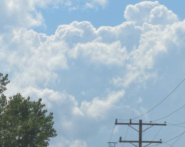
In cases where nearly half the histogram is occupied by a sprinkling of specular highlights, clipping the pixels is often the best and easiest solution. For the “Power lines” image, the 48 pixels in question carried essentially zero information. So I used “Colors/Exposure” to raise the white point, and then used “Tools/GEGL Operation/Clip RGB” to actually clip the channel information in the highlights (this time making sure the “Clip high pixel values” box was checked).
Some raw processors can output images with negative channel values. And previous edits using high bit depth GIMP might have produced negative channel values. If doing an “Auto/Stretch Contrast” on your base image layer makes the image a whole lot lighter in the shadows, the problem is negative RGB channel values. One solution is to use “Colors/Exposure” to move the black point to where you want it to be, and then clip the negative channel values. Here are two ways to clip negative channel values:
 After applying bilateral smoothing to the mask, micro contrast is restored.
Adding exposure compensation combined with an inverse grayscale mask does flatten micro contrast, which might or might not be desireable depending on your artistic intentions for the image. To restore micro contrast, try using an edge-respecting blur such as G’MIC’s bilateral smoothing filter. GIMP G’MIC doesn’t work on layer masks. A workaround is to to turn the unblurred mask into a selection, save the selection as a channel, and then drag the channel to the layer stack for blurring.
If the inverted grayscale masks were summarily clipped (as is the case when editing at integer precision), then the procedure described in this tutorial wouldn’t work.
Photographs taken in bright direct sunlight typically are of high dynamic range scenes, and the resulting camera file usually requires careful tone mapping to produce a satisfactory final image. High bit depth GIMP’s floating point floating point “Colors/Exposure” provides a very useful tool for dealing with this type of image, and of course is equally useful for any image where the goal is to raise the shadows and midtones without blowing out the highlights.
High bit depth GIMP’s floating point “Colors/Exposure” combined with a suitable layer mask can also be used to darken portions of the image, either by moving the upper left Value slider to the right (darkens the image by increasing contrast and also increases saturation; requires careful masking to avoid producing regions of solid black), or moving the lower right Value slider to the left (darkens the image by decreasing contrast, useful for de-emphasizing portions of the image).
This is a GIMP-specific tutorial. However, the same technique can be employed using the PhotoFlow raw processor and possibly other image editors that allow for 32-bit floating point processing using unbounded RGB channel values. The neat thing about using this technique in PhotoFlow is that PhotoFlow uses nodes, which allows for completely non-destructive editing of the inverted grayscale mask that’s used to recover the highlight detail after applying positive exposure compensation to raise the tonality of the shadows and midtones (even if you close and reopen the image, if you save the image’s PFI file).
The original tutorial this was adapted from can be found here and is reproduced courtesy of Elle Stone (https://ninedegreesbelow.com).
 GIMP Tutorial - Tone Mapping Using GIMP Levels (text & images) by Elle Stone is licensed under a Creative Commons Attribution-ShareAlike 3.0 Unported License.